Written by Brigitte Stenhouse, PhD student in History of Mathematics at the Open University.
The reactions I get when I tell people that my PhD is in History of Maths invariably involve some surprise: history and maths aren’t an obvious pairing, existing on separate sides of a perceived barrier between the humanities and the sciences. Beyond this, mathematics is commonly viewed as something static, unchanging, and the closest one can get to ‘truth’. Once you have given a mathematical proof, a mathematician’s job is done, right? So, what do we need history of mathematics for, when maths is the same now as it has always been?
However, the way we do mathematics today would be completely unrecognisable to Galileo, Newton, and their mathematical predecessors. Humans got along quite nicely for thousands of years before algebra was introduced (discovered? invented?), and although its utility was quickly recognised, it was plagued with philosophical objections for hundreds of years.
Mathematics is very much a human endeavour, and the progress of its development was and is strongly influenced by the idiosyncrasies of its practitioners. The transmission of knowledge between communities is affected by language barriers; political unrest; the circulation of journals, books and letters; transport and freedom of movement; and more. Thus, the history of mathematics can bring a different colour to the subject, and is a huge resource for alternative methods to solving problems, which students might not otherwise come across.
As such, when I was asked to give a Masterclass at Bletchley Park, I decided to run a workshop on the fluxional calculus, working through an extract from the 1736 English translation of Newton’s Method of Fluxions (below). BBC Bitesize was a great resource for finding out what the students would be expected to know, and what I would have to cover in the session before reading Newton. After revising equations of straight lines and giving examples of curves, we covered the relationship between tangents and gradients. We then looked briefly at Fermat’s method of drawing tangents to parabolas and discussed the benefits of having a general method which would work for all types of curves. This brought us neatly on to the calculus.
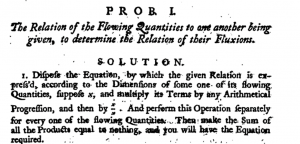
On first handing out the extract, I asked the students to underline all the words they didn’t recognise. After a few comments of “can I highlight the whole thing?”, there were soon conversations popping up about the strange typesetting of the ‘s’, and the difficulty of printing a fraction in the 18th century. Together we read through the extract and translated the rules we needed to follow into understandable modern English:
- Identify the variable unknowns in the equation (here only
 and
and  ).
). - Considering the variables one at a time.
- Put the terms in ascending order, depending on the power of the variable.
- Multiply by an arithmetic progression (here 1, 2, 3, …)
- Multiply each term by
 (or
(or  when considering etc.).
- Repeat for each variable.
- Set the sum of the resulting terms equal to 0.
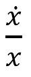
Newton’s method here gives an equation for what he calls the fluxions, ![]() and
and ![]() , in terms of
, in terms of ![]() and
and ![]() . However, in order to find the gradient of a line at a point we must go one step further; namely, we must rearrange the final equation into the form
. However, in order to find the gradient of a line at a point we must go one step further; namely, we must rearrange the final equation into the form ![]() .
.
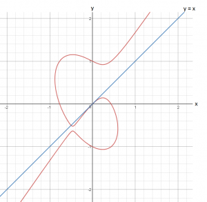
With the assistance of a table to fill out for each step of the calculation, we applied these rules to an example together, ![]() (graph below).
(graph below).
Once we had calculated ![]() , we checked our answer by calculating the gradient and plotting the tangent at the origin
, we checked our answer by calculating the gradient and plotting the tangent at the origin ![]() .
.
Hence, at this point, ![]() , and the equation of the tangent is
, and the equation of the tangent is ![]() . As we can see below, the line
. As we can see below, the line ![]() just touches our curve, as a tangent should.
just touches our curve, as a tangent should.
Having never taught a maths lesson before, I had been a little worried about making sure the extract was accessible in 2.5 hours. It was thus quite exciting for me to ask a question to the room, and receive answers (often correct!) from multiple directions. After working through a second example together, the students completed a worksheet on their own, applying Newton’s method to a selection of curves. I found it very interesting discussing with some of the students what happens to the constant in an equation when you differentiate it; some of them reintroduced the constant at the end of the calculation because they were unhappy with it completely disappearing. But on considering how a curve is transformed when a constant is added, they soon understood why this happened.
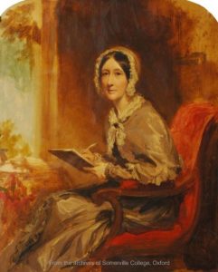
Beyond the mathematics, we looked at the feud between Newton and Leibniz owing to their almost simultaneous development of the calculus, and how this negatively impacted the transmission of future work between mathematical communities in France and the UK. I was thus able to introduce my own doctoral research on the work of Mary Somerville (1780-1872), who played a key role in the in the dissemination of what was termed ‘French analysis’ in the 19th century. Notably, she translated and adapted Pierre-Simon Laplace’s Traité de Mécanique Céleste in 1831 (retitling the work Mechanism of the Heavens), and advocated for the adoption of analysis in her 1834 book Connexion of the Physical Sciences. In both of these works she showcased the impressive results which can be gained by modelling natural phenomena using algebra and applying the calculus; for example predicting the motions of the planets and their moons, or even deducing the internal structure of the Earth.
I thoroughly enjoyed the chance to introduce these students to the history of mathematics, and look forward to re-running the session in the future!