
This blog post was written by Jemimah O’Regan as part of a Summer Research Project under the supervision and guidance of Dr. Elsen Tjhung.
Jemimah O’Regan completed her BSc (Hons) degree in Mathematics and Statistics with first-class honours at the Open University in the summer of 2022. She felt that the Summer Research Project was a great learning experience, and found that it allowed her to apply and develop new skills.
The following blog post demonstrates an example of random processes in nature, which can be described mathematically using probabilities.
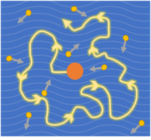
Consider, if you will, a particle placed inside of a box, which is then closed and filled with liquid. It is a tiny particle, so small as to be measured in micrometers, and it is subject to no forces other than the motion of the even smaller liquid molecules around it. If this box had a glass pane, and if one were able to see this tiny particle, one may note something curious. The particle will, of course, jostle and float as the water is poured into the box. Intuitively, though, one might expect that if one waits long enough, and keeps the box completely stationary, that the particle will eventually find a position to settle down in and stop moving. However, this is not what will happen. One could wait and wait, and yet this will not occur. This particle will continue to move.

In this simple case, it will not move due to gravity. There is nothing that the particle is attached to, no springs or strings acting on it and restraining or forcing its motion. There’s nothing obvious causing this motion, like the box being shaken or tilted, and it may leave one a little flummoxed that the particle refuses to settle.
Through examination, one may conclude that nothing larger than this particle is causing this motion, and one may even determine that it cannot be anything outside of the box making it move. Therefore, one may deduce, it must be something internal. Something very small, and an unobvious – uncommon – source of motion. The only thing inside of the box, other than the particle itself, is the liquid. The liquid which contains molecules even smaller than the particle – molecules which naturally move and collide in a manner that could be called random. When these molecules collide with the particle, they apply a force – ‘kicks’ – onto it, and those kicks push the particle in the liquid. These collisions happen all the time in other situations, but only really cause visible motion when the object being affected by the molecules is small enough to be displaced significantly by them.
This is the source of the particle’s continued motion, and the foundation of the concept of Brownian motion.
Brownian motion is, in a sense, an intersection between the fields of statistics and physics.
The particle’s motion can still be treated as a regular equation of motion, save in that it has a random component representing the random forces from the liquid molecules. As a result, its motion is not seen as deterministic, but rather, stochastic – that is, unlike many other cases in physics, one cannot guarantee exactly how the particle will move given the forces present on it.
Instead, due to the randomness introduced in the modelling, one may only draw conclusions on the motion the particle is likely to exhibit. This can be done using the concept of a probability distribution function from statistics, which provides the probability of (in this case) the particle being at a certain position at a certain time.
Say that the particle is at a certain position when one begins observation. At this point, which we take to be the beginning of the time scale, the particle is at its initial position with probability 1 – we know for certain where it is – and has the probability of taking any other position with value 0 – we know for certain where it isn’t.
After this first time point, however, the particle’s movement is not absolutely certain. It could start to move in any direction, it could collide with multiple particles and change directions and speed several times – as time increases, so too does the number of ways the particle could have moved since the beginning, and the number of positions it could end up in at the end of that time.

As time increases, the particle will explore the area of the box. Above is a representation of what the data over many such ‘runs’ of the physical situation and the probability distribution function at three times might look like for a particle constrained to move only in one dimension when the origin is zero – at small time values, the particle will most likely still be close to the origin, but as time increases, the particle’s probability of straying further away from its original position also increases. Similar reasoning holds for two dimensions.
There are many ways one can take this further – one can make the physical situation more complex (for example, by attaching the particle to a spring), or one could simulate the particle’s motion using computer software and analyze the data, one can find the trajectory of motion that the particle is most likely to take under certain conditions, and so on.
Motion is ubiquitous in life, and Brownian motion shows that it can occur even in situations one may assume would be stationary.